DDG-DA

Introduction

Due to the non-stationary nature of the real-world environment, the data distribution could keep changing with continuous data streaming. Such a phenomenon/problem is called concept drift (Lu et al. 2018), where the basic assumption is that concept drift happens unexpectedly and is unpredictable for streaming data.

To handle concept drift, previous studies usually leverage a two-step approach.

• Detect the concept drift.
• Adapt the model to the new data distribution.
  • Retrain the model
  • Fine-tune the model

Assumption

The latest data contains more useful information than the previous data.

Existing methods handle concept drift on the latest arrived data $Data^{(t)}$ at timestamp $t$ and adapt the forecasting model accordingly. The concept drift continues, and the adapted model on $Data^{(t)}$ will be used on unseen streaming data in the future (e.g., $Data^{(t+1)}$). The previous model adaptation has a one-step delay to the concept drift of upcoming streaming data, which means a new concept drift has occurred between timestamp $t$ and $t + 1$.

In this paper, we focus on predictable concept drift by forecasting future data distribution.

Background and Related Work

Streaming Data and Concept Drift

• Streaming Data

  $$\boldsymbol{X} = \{\boldsymbol{x}^{(1)}, \boldsymbol{x}^{(2)}, \cdots, \boldsymbol{x}^{(T)}\}$$

  where each element $\boldsymbol{x}^{(t)} \in \mathbb{R}^{m}$ is a $m$-dimensional vector.

  $$\boldsymbol{x}^{(t)} = [x^{(t)}_{1}, x^{(t)}_{2}, \cdots, x^{(t)}_{m}]$$

  Given a target sequence $\boldsymbol{y} = \{y^{(1)}, y^{(2)}, \cdots, y^{(T)}\}$ corresponding to $\boldsymbol{X}$.
• Algorithm are designed to build the model on historical data $\{\boldsymbol{x}^{(i)}, y^{(i)}\}_{i=1}^{t}$ and predict the future data $\boldsymbol{x}^{(t)}$ and forecast $\boldsymbol{y}$ on unseen streaming data $D^{(t)}_{test} = \{\boldsymbol{x}^{(t)}, y^{(t)}\}_{t=1}^{\mathcal{T}}$.
• Assume $(\boldsymbol{x}^{(t)}, y^{(t)}) \sim p_t(\boldsymbol{x}, y)$, where $p_t(\boldsymbol{x}, y)$ is the data distribution at timestamp $t$. Generally, $p_t(\boldsymbol{x}, y)$ is non-stationary and keeps changing with time $t$, which is called concept drift. Formally, the concept drift between two timestamps $t$ and $t + 1$ can be defined as

  $$\exists \boldsymbol{x}: p_t(\boldsymbol{x}, y) \neq p_{t+1}(\boldsymbol{x}, y)$$

• Adapting models to accommodate the evolving data distribution.

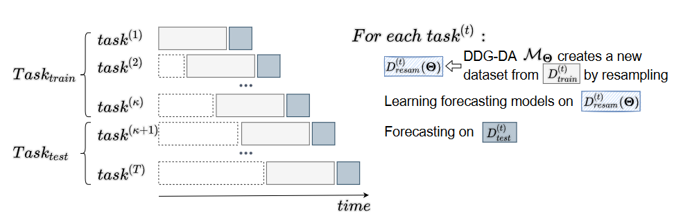
  $$\arg \min_{f^{(t)}, f^{(t+1)}, \dots, f^{(t+\mathcal{T})}} = \sum_{i=t}^{t+\mathcal{T}} \mathcal{l}(f^{(i)}(\boldsymbol{x}^{(i)}), y^{(i)})$$

  where $f^{(i)}$ is the model learned from data $D^{(i)}_{train} = \{\boldsymbol{x}^{(i)}, y^{(i)}\}_{i=t-k}^{t-1}$ and $\mathcal{l}$ with windows size $k$.

The Categorization of Concept Drift

• Measure the changing speed
  • abrupt: the data distribution changes suddenly
  • gradual: the data distribution changes slowly
• recurring or non-recurring
  • recurring: the data distribution changes periodically and the period is fixed
  • non-recurring: the data distribution changes periodically and the period is not fixed

Related Work

Previous Work

• Use a small trigger window to detect the concept drift and adapt the model to the new data distribution after the concept drift happens.
• Incremental adaptation.

DDG-DA

• Predict and adapt before the concept drift happens.
• Model-agnostic.

Method Design

Overall

Learning

• DDG-DA (annotated as $\mathcal{M}_{\Theta}$) models the concept drift and predict $p_{test}^{(t)}(\boldsymbol{x}, y)$.
• $\mathcal{M}_{\Theta}$ art like a weightd data sampler to resample on $D^{(t)}_{train}$ and generate a new training set $D^{(t)}_{resam}(\Theta) \sim p_{resam}^{(t)}(\boldsymbol{x}, y; \Theta)$.
• Minimize the gap between $p_{test}^{(t)}(\boldsymbol{x}, y)$ and $p_{resam}^{(t)}(\boldsymbol{x}, y; \Theta)$.
• During the training process,

Forecast

• Given $task^{(t)} \in Task_{test}$, the forecast model is trained on $D^{(t)}_{resam}(\Theta)$ and forcast on $D^{(t)}_{test}$.
• $p^{(t)}_{resam}(\boldsymbol{x}, y; \Theta)$ is more similar to $p^{(t)}_{test}(\boldsymbol{x}, y)$ than $p^{(t)}_{train}(\boldsymbol{x}, y)$. So the preference of model $f^{(t)}$ on $D^{(t)}_{resam}(\Theta)$ is more similar to $f^{(t)}$ on $D^{(t)}_{test}$ than $f^{(t)}$ on $D^{(t)}_{train}$.

Example

To handle the concept drift in data, we retrain a new model each month (the rolling time interval is 1 month) based on two years of historical data.

Each chance to retrain a new model to adapt the concept drift is called a task. For example, the task $task^{(2011/01)}$ contains $D^{(2011/01)}_{train}$ from 2009/01 to 2010/12 and $D^{(2011/01)}_{test}$ in 2011/01.

Set all $D^{(t)}_{test}$ range from 2011 to 2015 and DDG-DA will evaluated on $Task_{test}$ range from 2016 to 2020.

Model design and learning process

• Build a set of tasks $Task_{train} = \{task^{(1)}, task^{(2)}, \cdots, task^{(\mathcal{T})}\}$.
• The goal of the learned DDG-Da is to improve the performance of the forecast model on $Task_{test} := \{task^{(\mathcal{T}+1)}, task^{(\mathcal{T}+2)}, \cdots, task^{(T)}\}$.

Feature Design

Objective Function

• $\mathcal{M}_{\Theta}$ accepts the extracted feature and outputs the probability distribution $p_{resam}^{(t)}(\boldsymbol{x}, y; \Theta)$.
• To minimize the gap between $p_{resam}^{(t)}(\boldsymbol{x}, y; \Theta)$ and $p_{test}^{(t)}(\boldsymbol{x}, y)$, we use the KL divergence as the objective function.

  $$L_{\Theta}(task^{(t)}) = D_{KL}(p_{test}^{(t)}(\boldsymbol{x}, y) || p_{resam}^{(t)}(\boldsymbol{x}, y; \Theta))$$

  or

  $$L_{\Theta}(task^{(t)}) = \mathbb{E}_{\boldsymbol{x} \sim p_{test}^{(t)}(\boldsymbol{x})} \left[ D_{KL}(p_{test}^{(t)}(y|\boldsymbol{x}) || p_{resam}^{(t)}(y|\boldsymbol{x}; \Theta)) \right]$$

  where $D_{KL}$ is the KL divergence. $||$ is the divergence between two distributions. $\mathbb{E}_{\boldsymbol{x} \sim p_{test}^{(t)}(\boldsymbol{x})}$ is the expectation over the test data distribution $p_{test}^{(t)}(\boldsymbol{x})$.
• Normal distribution assumption is reasonable for unknown variables and often used in maximum likelihood estimation. So we assume $p_{test}^{(t)}(y|\boldsymbol{x})$ and $p_{resam}^{(t)}(y|\boldsymbol{x}; \Theta)$ are normal distributions.

  $$p_{test}^{(t)}(y|\boldsymbol{x}) = \mathcal{N}(y^{(t)}_{test}(\boldsymbol{x}), \sigma)$$

  $$p_{resam}^{(t)}(y|\boldsymbol{x}; \Theta) = \mathcal{N}(y^{(t)}_{resam}(\boldsymbol{x}; \Theta), \sigma)$$

  Tips

  $y^{(t)}_{resam}(\boldsymbol{x}; \Theta)$ is the expectation of $y$ under the predicted distribution $p_{resam}^{(t)}(y|\boldsymbol{x}; \Theta)$.

• According to the definition of KL divergence, we have

  $$L_{\Theta}(task^{(t)}) = \frac{1}{2} \sum_{(\boldsymbol{x}, y) \in D^{(t)}_{test}} || y^{(t)}_{resam}(\boldsymbol{x}; \Theta) - y||^2$$

  Summarize losses of all tasks, we have

  $$\Theta^{\star} = \arg \min_{\Theta} \sum_{task^{(t)} \in Task_{train}} L_{\Theta}(task^{(t)})$$

Optimization

• Build a regression proxy model $y_{proxy}^{(t)}(\boldsymbol{x}; \phi)$ to approximate $y^{(t)}_{resam}(\boldsymbol{x}; \Theta)$.

  $$\phi^{(t)} = \arg \min_{\phi} \sum_{(\boldsymbol{x}, y) \in D^{(t)}_{train}(\Theta)} || y_{proxy}^{(t)}(\boldsymbol{x}; \phi) - y||^2$$

Code

References

• Arxiv